
Skatelligence V0 is the first protoype of Skatelligence. This page will give an in depth overview of how this first protype works.
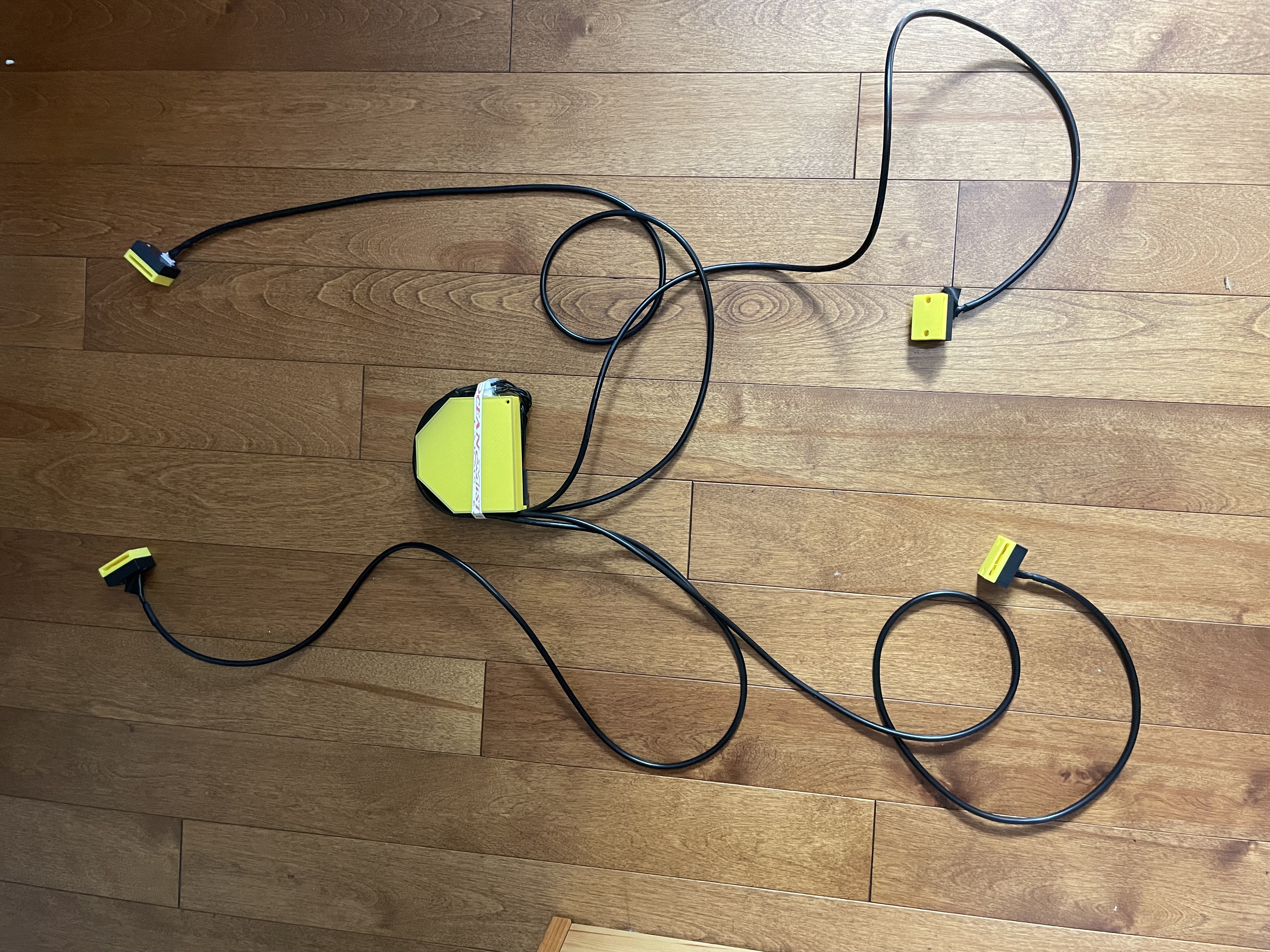
Skatelligence V0 consists of 5 main modules. 1 being the central module mounted to the skater's lower back, and the other 4 being accelerometers connected to each of the skaters wrists and skates. All 4 of the smaller modules are connected to the main module using wires, and the main module connects to a computer using wifi.
The main module consists of the following components
Each of the smaller modules consists of the following components:
The following images show the electrical connections of Skatelligence V0, as well as the two types of modules with the covers removed.
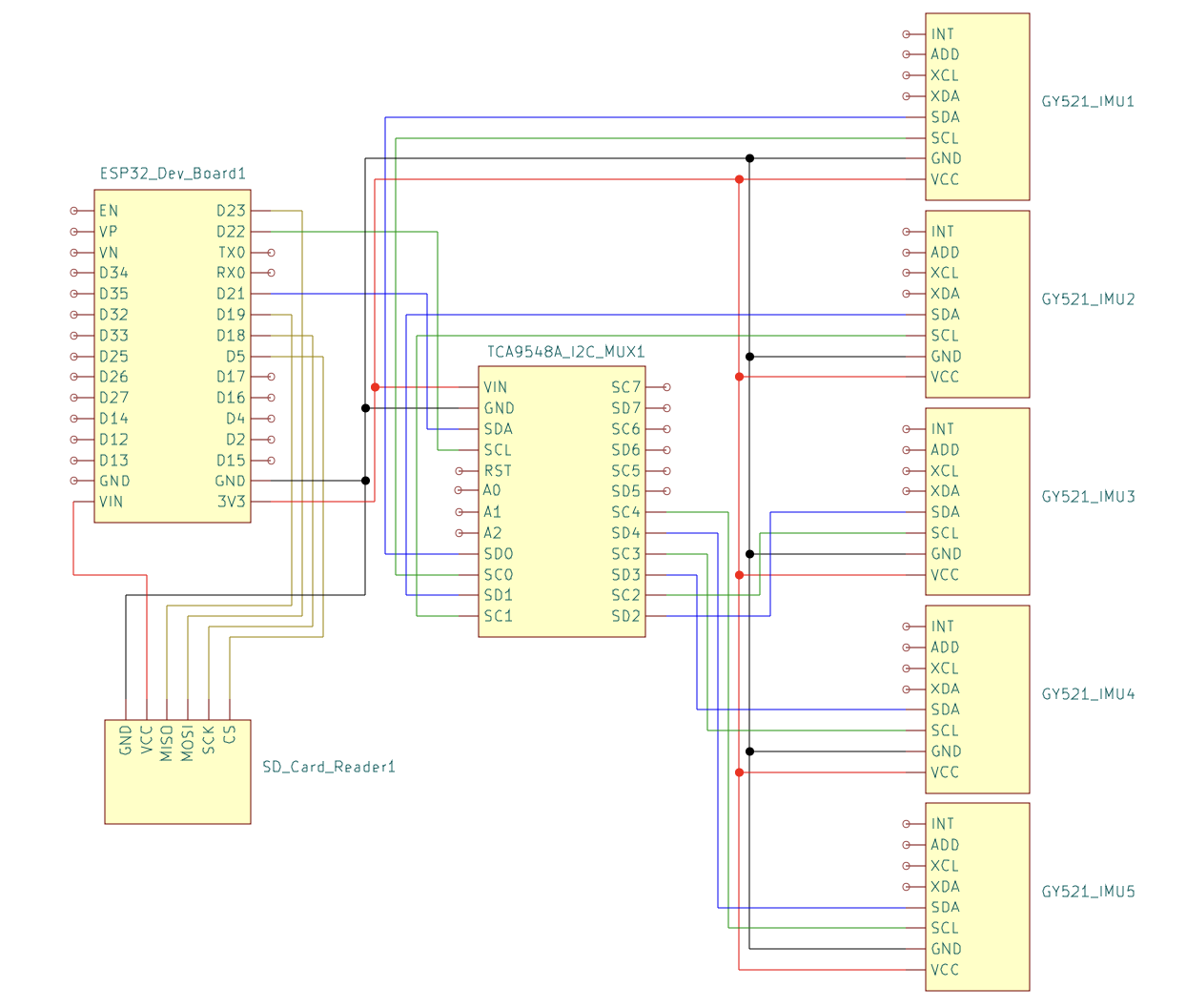
Electrical Schematic
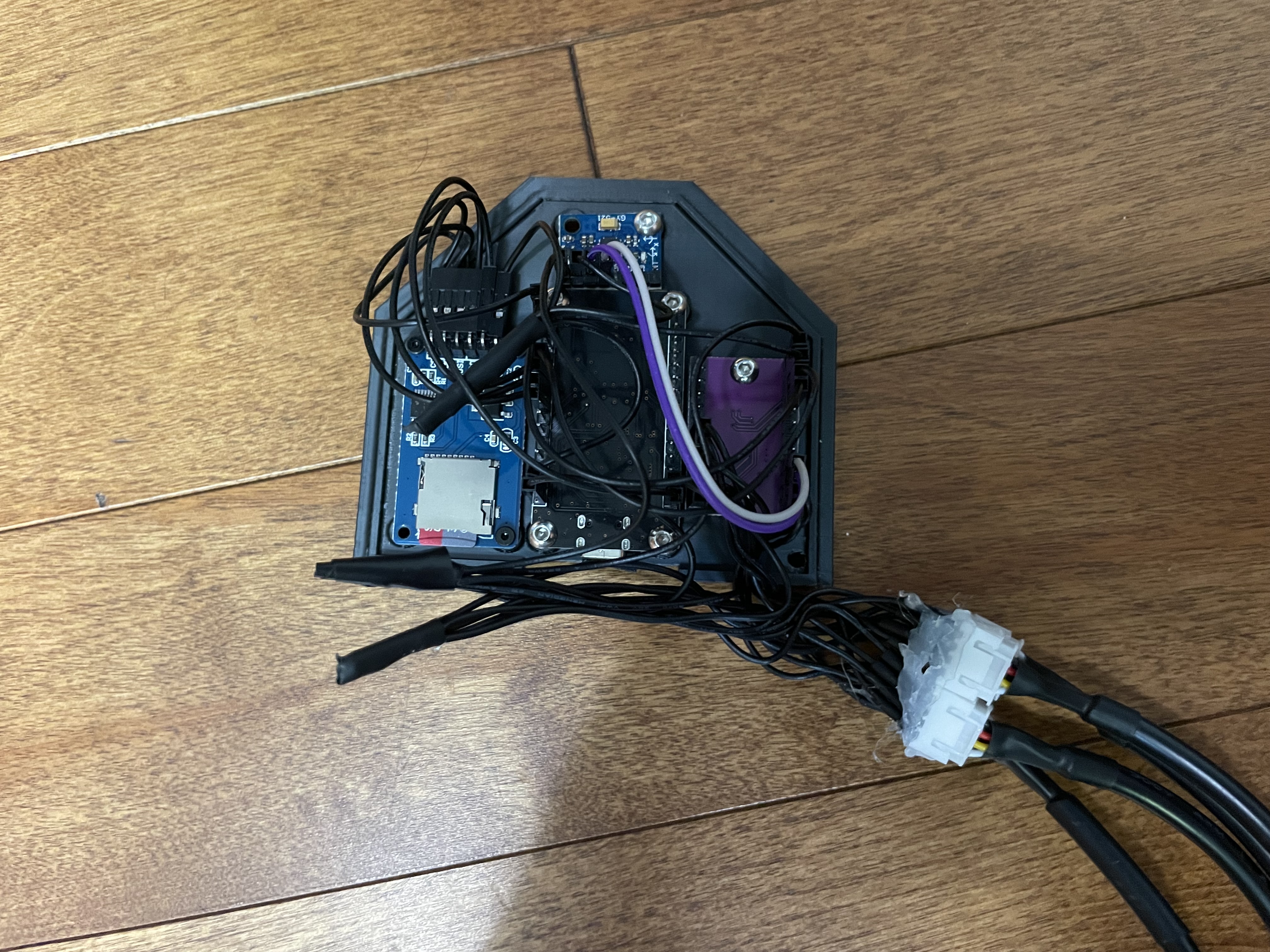
Main Module with Lid Removed
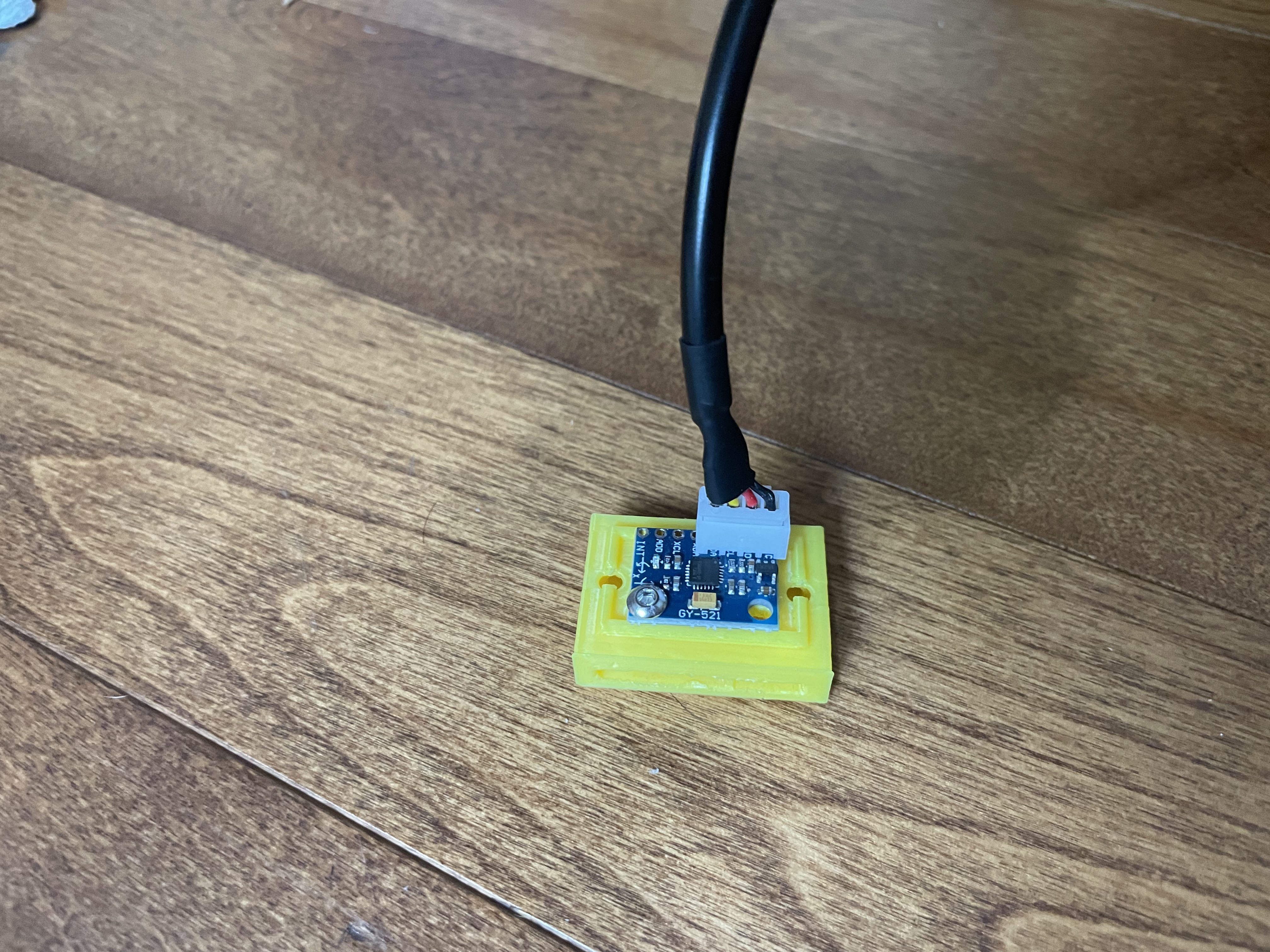
IMU Module with Lid removed
The ESP32 microcontroller is configured to interface with five GY-521 IMUs through an I2C multiplexer. Each IMU contains an MPU6050 sensor that measures three-dimensional linear acceleration and rotational velocity. The data collection is handled by one core of the ESP32, which collects all 6 measurements from all 5 sensors at a frequency of exactly 100 Hz. The measurements are read and stored as signed 16 bit integers. The readMPU6050, as seen in the code snippet, is responsible for the reading of the sensor
void readMPU6050(int16_t* Ax, int16_t* Ay, int16_t* Az, int16_t* Gx, int16_t* Gy, int16_t* Gz) {
    Wire.beginTransmission(0x68); // MPU6050 address
    Wire.write(0x3B);             // Starting register for Accel Readings
    Wire.endTransmission(false);
    Wire.requestFrom(0x68, 14, true); // Request 14 registers
    *Ax = Wire.read() << 8 | Wire.read();
    *Ay = Wire.read() << 8 | Wire.read();
    *Az = Wire.read() << 8 | Wire.read();
    Wire.read(); Wire.read(); // Skip temperature
    *Gx = Wire.read() << 8 | Wire.read();
    *Gy = Wire.read() << 8 | Wire.read();
    *Gz = Wire.read() << 8 | Wire.read();
}
In order to enable batch transfering of data to the server. 100 complete readings from all 5 sensors are stored in a binary file before being transfered All data measurements are 2 bytes, and are stored in the following format.
Denote each sensor reading as #MdR: Where # is the sensor number (0-4), M is the measurement (A for Accel or G for Gyro), d is the direction (x, y, or z), and R is the reading number (0-99) The data is then stored in the following order, with no padding between the readings:
0Ax0, 0Ay0, 0Az0, 0Gx0, 0Gy0, 0Gz0, 1Ax0, ..., 1Gz0, ..., 4Gz0
0Ax1, 0Ay1, 0Az1, 0Gx1, 0Gy1, 0Gz1, 1Ax1, ..., 1Gz1, ..., 4Gz1
0Ax99, 0Ay99, 0Az99, 0Gx99, 0Gy99, 0Gz99, 1Ax99, ..., 1Gz99, ..., 4Gz99
These 6KB files are stored locally on the SD card with file names 0.bin, 1.bin, 2.bin ... The files will remain on the SD card until the system is rebooted, at which point the SD card is wiped to begin a new recording.
See the function readData for the implementation of this logic. Note that some lines have been commented out for the sake of brevity. Please see the GitHub repo under Related Links for the full code
void readData(void * parameter) {
    TickType_t xLastWakeTime;
    const TickType_t xTimeIncrement = pdMS_TO_TICKS(POLL_INTERVAL_MS);

    //Initialize other variables

    while (1) {
        // Wait until xTimeIncrement after xLastWakeTime
        vTaskDelayUntil(&xLastWakeTime, xTimeIncrement);

        if (!file){
            String fileName = "/" + String(fileNumber) + ".bin";
            file = SD.open(fileName, FILE_WRITE);
            if (!file) {
                Serial.println("Failed to open file for writing");
            } else {
                Serial.println("File opened successfully: " + fileName);
            }
        }

        for (int i = 0; i < 5; i++) {
            int16_t Ax, Ay, Az, Gx, Gy, Gz;
            tcaSelect(i);
            readMPU6050(&Ax, &Ay, &Az, &Gx, &Gy, &Gz);
            //Write data to file
        }

        pollCount++;

        // Check if this file is done
        if (pollCount >= POLLS_PER_FILE) {
            file.close();
            lastCompletedFile = fileNumber; // Update the last completed file index
            fileNumber++;
            pollCount = 0;
        }
    }
}
After the data collection core of the ESP32 writes a file to the SD card, the other core attempts to upload it to a local server via HTTP. If the ESP32 detects a loss of internet connectivity, it continues to store data locally on the SD card and resumes uploading when connectivity is restored. This functionality is managed by checking the Wi-Fi connection status before each upload attempt and implementing a retry mechanism if the connection fails. The local server receives these files over the network, and processes the data, as will be outlined in the next section.
Before identifying the specific jumps in the collected data, the raw binary files generated by the main unit must be processed. This processing involves two primary steps: data extraction, and filtering. The first of these steps is handled by the Python function read_file, as seen in the code snippet. This function reformats the data into a 100x30 numpy array, each column representing one stream of data (e.g. Sensor 0, Acceleration X). The data is then scaled to the appropriate units (Gs for acceleration and deg/s for rotational velocity)
def read_file(file_path):
    # Scale the data and return that array
    if file_path:
        data = np.fromfile(file_path, dtype=np.int16)
        if data.size == 0:
            print(f"Warning: {file_path} is empty.")
            return None
        data = data.reshape((-1, SENSOR_COUNT * 6))
        scale_vector = np.tile(np.hstack([ACCEL_SCALE]*3 + [GYRO_SCALE]*3), SENSOR_COUNT)
        scaled_data = (data / 32768.0) * scale_vector
        return scaled_data
The final step of the data processing is to apply a low-pass filter. This helps to reduce the noise in the raw sensor readings, and leads to more reliable jump identification. In particular, we are using a low-pass 6th order Butterworth filter, as implemented in the function apply_low_pass_filter. This filtered data is then converted back into the file format used for the raw data, and stored in the same manner.
def apply_low_pass_filter(data, cutoff, fs, order):
    nyq = 0.5 * fs  # Nyquist Frequency
    normal_cutoff = cutoff / nyq  # Normalize the frequency
    b, a = butter(order, normal_cutoff, btype='low', analog=False)  # Get filter coefficients
    filtered_data = filtfilt(b, a, data, axis=0)  # Apply filter
    return filtered_data
The jump classification is performed using two steps. First all jumps are identified, then the jumps are passed into an AI model to be classified. In order to detect jumps, we have determined that a sequence of IMU readings contains a jump if and only if it meets the following criteria:
If the above criteria is met, we take the jump to end 0.3 seconds after the landing phase and begin 1.5 seconds before that end. If a jump has been identified, the 150 readings are extracted and stored in a 9KB binary file. Using this method, we were able to obtain a jump identifcation accuracy of essentially 100%. A simplified implementation of this algorithm can be seen here (For the complete script refer to the GitHub):
def detect_jumps(x_accel_data, start_time_offset):
    #Initialize variables
    for i in range(len(x_accel_data)):
        # If the first file has been analyzed and it is not currently in the middle of a jump, stop.
        # This is because the second file will be analyzed in the next call to the function anyways
        if i >= READINGS_PER_FILE and state == STATE_GROUNDED:
            return jumps

        x_accel = x_accel_data[i]
        current_time = start_time_offset + i / SAMPLING_RATE  # Calculate the current time in seconds
        if state == STATE_GROUNDED:
            # If accel goes above threshold, register a takeoff
            if x_accel > HIGH_THRESHOLD:
                state = STATE_TAKEOFF
                jump_start = i
                jump_start_time = current_time

        elif state == STATE_TAKEOFF:
            # If accel drops below low threshold, set to air state
            if x_accel < LOW_THRESHOLD:
                state = STATE_IN_AIR

        elif state == STATE_IN_AIR:
            current_duration = current_time - jump_start_time  # Calculate the current duration of the jump

            # If high acceleration spike after being in the air, they have landed
            if x_accel > HIGH_THRESHOLD:
                jump_end = i
                jump_end_time = current_time
                if MIN_JUMP_DURATION <= current_duration <= MAX_JUMP_DURATION: # Ensure it within acceptable time range
                    jumps.append((jump_start_time, jump_end_time))
                state = STATE_GROUNDED

            # Reset if the jump exceeds the maximum duration
            if current_duration > MAX_JUMP_DURATION:
                state = STATE_GROUNDED

        return jumps
For our initial prototype of the Skatelligence V0, we mounted the device on a skater to collect data during the execution of various single jumps. Due to the time constraints of prototype testing, we only recorded single jumps from a single skater. Despite this limitation, the dataset includes a comprehensive representation of single jump types. Moving forward, expanding the dataset to include multiple skaters and more complex jumps with additional rotations is planned to improve model robustness and generalizability.
We settled on using a Recurrent Neural Network (RNN), utilizing Long Short-Term Memory (LSTM) units, to perform the jump classification. This choice was generally made for the following reasons:
The model that we are using contains 30 input features (corresponding to 6 readings for each of 5 sensors). It contains 4 hidden layers each with a size of 50. Through experiementation, we determined that moving beyond this did not improve identification accuracy. The output is passed into a fully connected layer, which classifies the jump into 1 of 6 categories (Salchow, Toe loop, Loop, Flip, Lutz, Axel).
The model was developed using PyTorch, and the strucutre of it can be seen in the Python code on the left
class JumpClassifier(nn.Module):
def __init__(self):
    super(JumpClassifier, self).__init__()
    self.lstm = nn.LSTM(input_size=30, hidden_size=50, num_layers=4, batch_first=True)
    self.fc = nn.Linear(50, 6)  # 6 categories

def forward(self, x):
    x, _ = self.lstm(x)
    x = x[:, -1, :]  # Get last time step
    x = self.fc(x)
    return x
The data set we had collected was split into training and testing data. After training the model on the training data, it was able to achieve a successfull identification on the testing data ~80% of the time. We believe that this number will signficiantly improve, and generalize to other skaters/jumps after we collect more data. The model was tested using the following Python code:
tensor_data = torch.Tensor(data)
tensor_labels = torch.LongTensor(labels)

X_train, X_val, y_train, y_val = train_test_split(tensor_data, tensor_labels, test_size=0.3, random_state=42)
train_dataset = TensorDataset(X_train, y_train)
val_dataset = TensorDataset(X_val, y_val)

train_loader = DataLoader(train_dataset, batch_size=16, shuffle=True)
val_loader = DataLoader(val_dataset, batch_size

criterion = nn.CrossEntropyLoss()
optimizer = torch.optim.Adam(model.parameters(), lr=0.001)

for epoch in range(200):  # Number of epochs
    for inputs, labels in train_loader:
        optimizer.zero_grad()
        outputs = model(inputs)
        loss = criterion(outputs, labels)
        loss.backward()
        optimizer.step()
    print(f'Epoch {epoch+1}, Loss: {loss.item()}')